Basic Usage
Overview
If this is the first time you are using Trodes, chances are you are not yet at the point where you are ready to record from an animal but still need to figure out how to use Trodes before you get to that point. Or perhaps you are simply evaluating the software. In these cases, we highly recommend that you download this previously recorded sample dataset in order to have real neural data to visualize as you are exploring the controls. You can also use the built-in simulator sources, but they are not very realistic signals. In the examples below, we will use the 16-channel recording from the downloaded example file. The download contains two files: 1) example_recording.rec and 2) example_recording.trodesconf.
Main Interface
Upon opening Trodes you will be greeted with an intro page that will allow you to help you navigate the program. From this menu, you can create a workspace, open a pre-existing workspace, or open a playback file. Each menu will expand when you click on it and show sub-options, such as the most recently used workspaces for quick access.
For our example, we will start by opening up a previously recorded file. Click on “Open Playback File” and select “Browse”. Then, browse to and select example_recording.rec. Once you select the file, the accompanying workspace located in the same folder and with the same name (example_recording.trodesconf) will be loaded and you will see the main interface screen:
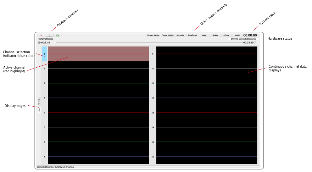
Trodes Main Display
Each nTrode, or bundle of channels, is assigned a number starting from one. These numbers are displayed to the left of the traces. In this recording, each nTrode only has one channel. After loading, you will notice that the first nTrode number has a blue highlight, indicating that it is one of the channels currently selected. At the top of the screen, there is a row of buttons (labeled quick access controls). These buttons are used to perform some of the most common operations. On the left side of the screen there are two tabs labeled “Tr 1-16” and “Aux”. These are display pages that allow the channels to be distributed across multiple pages to prevent overcrowding when many channels are present.
Source Control
In the top menubar, click on “Connection” and hover your mouse over “Source”. You will notice that “File” is already selected, indicating that the current source is from a previously recorded file. If you hover over “SpikeGadgets”, you will notice that there are two ways of connecting to the SpikeGadgets MCU (either USB or ethernet), and one way to connect to the Logger Dock (Dock (USB)). For now, we will leave the source as “File”, but during normal recording sessions you would set the source from this menu before data acquisition is initiated.
To start streaming data from the selected source, select Connection->Stream from source. This will initiate data acquisition from the selected source. A vertical white line will move from left to right on the trace display panels, indicating where the most recent data are being plotted:
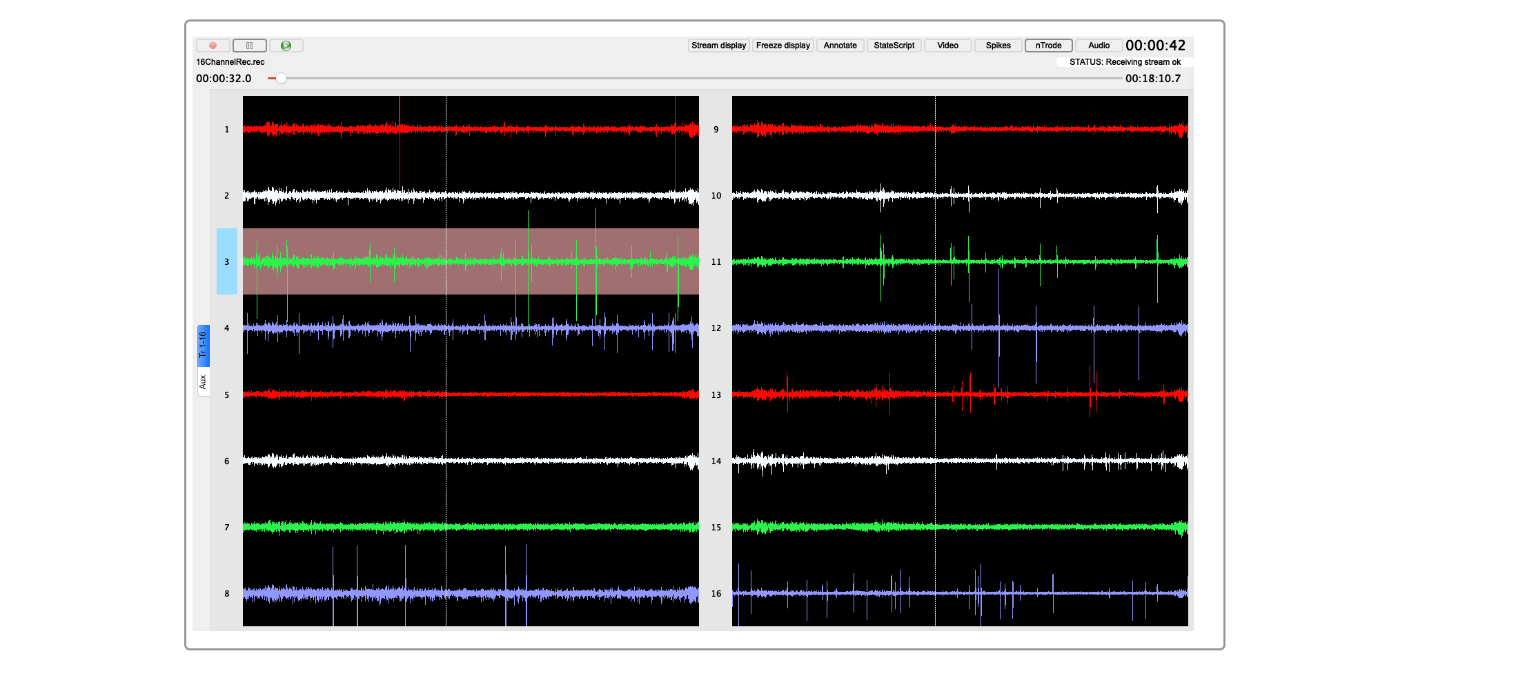
Streaming in Trodes
During file playback, you can pause playback by either pushing the pause button at the top of the screen or selecting File->Pause. During live acquisition, you can stop acquiring data from the source by selecting Connection->Disconnect. Doing this during playback simply pauses playback and resets the file to the beginning of the recording.
The nTrode Panel
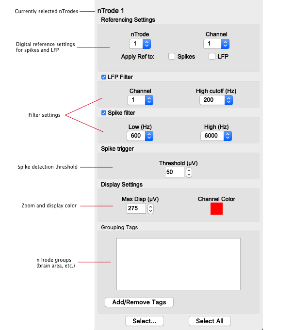
Press on the “nTrode” button among the quick access controls. This will make a control panel appear that is used to set important settings for all currently selected nTrodes. The panel will stay open until you close it, and many users prefer to keep it open in a corner of the screen.
nTrode panel.png
The panel is organized into separate sub-panels. Each sub-panel controls a different category of processing or display options for the currently selected nTrode. You can turn on/off the spike and LFP filters by toggling the corresponding checkboxes. You can apply a digital reference by selecting any channel from another nTrode that will be subtracted from the signals in the selected nTrode(s). You can also change spike trigger threshold, display settings, and channel groupings. Any changes you make are applied immediately. It is important to note that when you are recording data, making changes in the nTrode panel does not affect how the data are saved– all data are saved as continuous broadband signals at full sampling rate and with no digital reference applied. The settings are for visualization and online processing only. At any time, you can save the changes made to the workspace by going to File->Workspace->Save workspace as…
Keep the nTrode panel open. Back on the main interface, click on a different nTrode (either by clicking the number or the trace). You will notice that the blue highlighting will shift to the clicked channel, and that the background of that channel will be red. Also, the nTrode settings panel will update to display the settings for that nTrode. The red highlight indicates that this channel is the “active” channel (unlike the blue highlighting, only one channel can be active at a time). The active channel is streamed to your audio device and also defines which nTrode is displayed in the “Spikes” panel (see below).
In the nTrodes panel, toggle the checkbox for the Spike Filter group. You will notice that unchecking this box turns off the spike filter for the selected channel, and you will see more low-frequency oscillations in the main window. If audio is available on your computer, you will also hear low-frequency rumbling. If you want to change settings for multiple nTrodes simultaneously, either shift-click or control-click multiple channels in the main window to select multiple nTrodes. You can also select nTrodes by selecting pre-defined groups at the bottom of the nTrode panel, or you can press the “Select All” button to select all of the nTrodes. Feel free to play around with the different settings in the nTrode panel before moving on.
The Spikes Panel
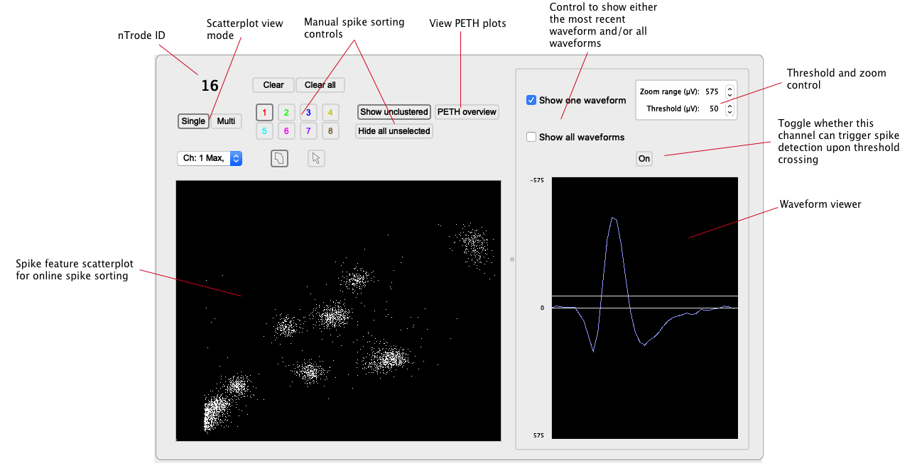
Press the “Spikes” button in the quick access controls. This will open up a window that displays information about detected spikes from the active nTrode. If you click on a different nTrode in the main window, the Spikes window will automatically update to show spike information for the selected nTrode. Just like the nTrode panel, the spikes window will remain open until you close it. All settings (including cluster bounds) are persistent when you close the window).
Trodes Spikes window
On the left side of the Spikes window, you will see a 2-D scatter plot that plots two features of each spike. With the 16-channel file, each nTrode has only one channel. In this case the scatter plot will plot the maximum and minimum amplitude of each spike. Above the scatter plot are buttons that are used to draw polygons around individual clusters for online spike sorting. Polygons can be saved and loaded from the File menu. You can also open up a PETH analysis window if a PETH trigger has been defined.
On the right side of the Spikes window, the spike waveforms are plotted. You can either display just the most recent spike, or all of the spikes (color coded by clusters if they have been defined).
If the nTrode has more than one channel, the Spikes window looks a bit different. All waveforms in the nTrode are displayed on the side of the window. Also, the Multi view button becomes enabled, allowing the user to see all pair-wise scatterplots simultaneously, where each plot shows the peak spike amplitude for two of the channels in the nTrode. Below, a spike window for a tetrode (four channels) is shown with Multi view enabled (credit to Anna Gillespie from the Frank lab for the dataset):
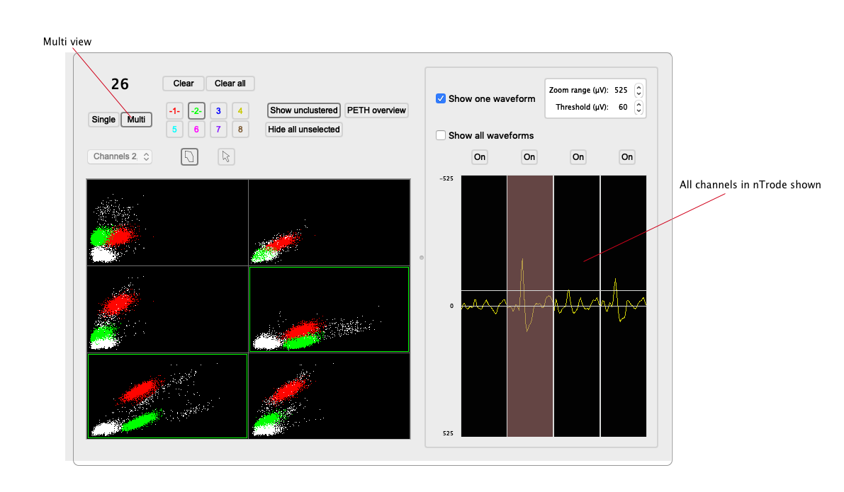
SpikeWindowTetrode.png
Recording
Now that we have covered some of the basic controls, the next step is to create a recording. Since this can not be done when you are in playback mode, we will need to exit playback mode and return to the intro menu. To do this, select File->Close file. If you made any changes to the workspace, you will be asked if you want to save them before the file is closed.
In the intro menu, click on “Open Workspace”, then “Browse”. Navigate to the downloaded example_recordng.trodesconf file. Normally you will need to choose a workspace that exactly matches the hardware configuration, but since we are simply going to simulate fake data it doesn’t matter right now.
Once the workspace is loaded, select Connection->Source->Simulation->Signal Generator (w/spikes). Then, select Connection->Stream from source. You will notice that fake spike data is now streaming on all channels. We will pretend this is real data coming from an animal, and that you are ready to start your recording.
You may notice that near the upper left corner of the window it says “No file open” to indicate that you have not created a file yet. Select File->New recording. This will open up a save dialog with a suggested filename and location. The default location and prefix of the filename are defined in the loaded workspace, and can be modified using the workspace editor (see below). The second part of the default filename is today’s date followed by the time. Choose a good location to create the file, and click “Save”.
Now, you will notice that the top of the window has a lot more information displayed. From left to right, you will see 1) The name of the open file, 2)The size of the file and space available, and 3)A bright yellow bar stating that the recording is paused.
To start the recording, select File->Record. For quick access, you can also click the record button at the top of the window. Recording has now begun. You will notice that the yellow bar changed color to green to make it very obvious that you are now collecting data. Now, hit the pause button. The recording has now paused, but the clock from hardware continues to increase. If you hit record again, recording will start again, but there will be a gap in timestamps during the time that recording was paused. When you are ready to end the recording completely, select File->Close file. To disconnect from the source, first select Connection->Disconnect. Then select File->Workspace->Close to return to the intro menu. You can now play back the recorded file using the “Open Playback File” menu if you want. You can also export data from the recording file to analyze in Matlab or Python (see Exporting Data section).
Creating/Opening a Workspace
In it’s most basic form, Trodes is run by opening a workspace file (extension .trodesconf). These files are used by Trodes to save experimental configuration settings, including what kind of hardware will be streaming data from and how that data will be displayed in Trodes.
You can create you own by following the instructions outlined in the Working with Workspaces section of the wiki.
Re-using a Workspace
After you have your hardware and computer set up, you can simply re-open a previously created workspace. To open a workspace, simply press the “Open Workspace” button and select the “Browse” option, or click Ctrl-o, and open the desired workspace file.
Impedance Measurement
Trodes is also capable of measuring the impedance of connected probes and can be found under the follow menu:
View > Tools > Impedance Measurement
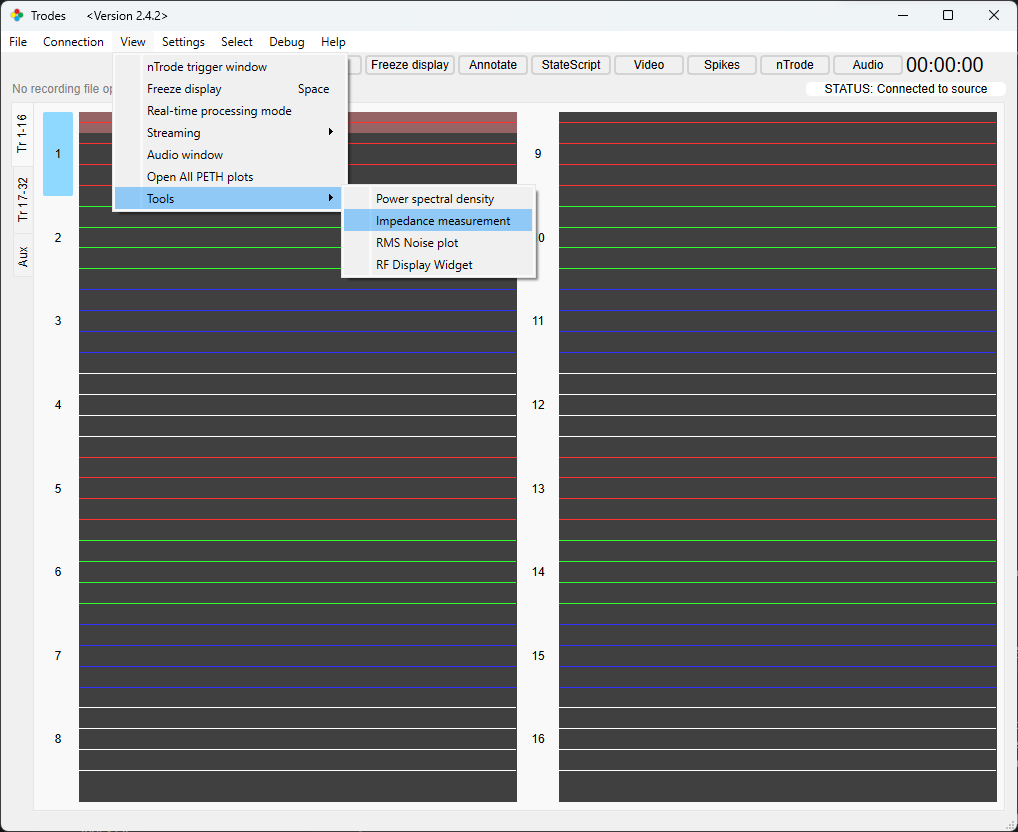
The Impedance measurement tool is a new tool that is still under active development, and will have expanded features in the future. Currently it is capable of returning impedance values for each channel in the workspace regardless of nTrode assignment. The semi-automated electroplating feature that can be seen in the interface is not currently available as of Trodes 2.5.0, but is planned for a future release.
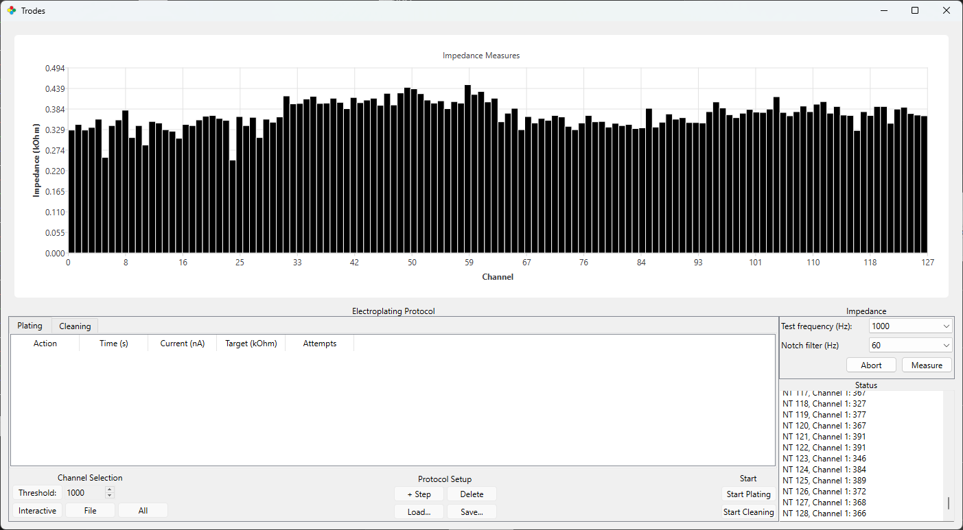
Currently, impedance values are listed in the right sidebar, but cannot be exported as a text file. This feature will be available in a future release.